Understanding Martingales, Mean Reversion, and Delta Hedging in Financial Modeling

In exploring the nuances of financial modeling, we delve into concepts such as martingales, mean reversion, real-world versus risk-neutral probabilities, and delta hedging strategies. This comprehensive guide aims to elucidate these concepts, providing clear explanations and practical insights for students and professionals alike.

Martingales vs. MA(1) Processes in Stock Modeling

Understanding the fundamental properties of stochastic processes like martingales and Moving Average processes (MA(1)) is crucial when modeling stock prices.

Martingales are stochastic processes where the conditional expected future value, given all prior information, equals the present value. Mathematically, for a process ( X_t ), this is represented as: [ E[X_{t+1} | X_t, X_{t-1}, ...] = X_t ]

In contrast, an MA(1) process incorporates past shocks into the current value: [ X_t = mu + epsilon_t + theta epsilon_{t-1} ] where ( epsilon_t ) is white noise, ( theta ) is the coefficient, and ( mu ) is the mean.

The key distinction lies in predictability. MA(1) processes have a predictable component due to ( theta epsilon_{t-1} ), whereas martingales do not have any predictable movements based on past information. Therefore, proposing an MA(1) structure is inappropriate if a stock price is truly a martingale. The econometrician's claim of MA(1) structure in a martingale stock price contradicts the mathematical properties of martingales.

Mean Reversion in Stock Prices and Martingales

Mean reversion suggests that a stock price tends towards a long-term average over time. The expected change in a mean-reverting process is:
[ E[X_{t+1} - X_t | X_t] = alpha (mu - X_t) ] where ( mu ) is the long-term mean and ( alpha > 0 ) is the speed of reversion.

This indicates a predictable drift towards the mean ( \mu ), violating the martingale property where: [ E[X_{t+1} - X_t | X_t] = 0 ]

Therefore, a stock price exhibiting mean reversion cannot be a martingale. The technical analyst's assertion of mean reversion in a martingale stock price is mathematically incompatible.

Real-World vs. Risk-Neutral Probabilities

In financial modeling, distinguishing between real-world (physical) and risk-neutral probabilities is vital, especially in derivative pricing.

• Real-World Probabilities: These reflect actual probabilities based on historical data, including investors' risk preferences and expected returns mu: 

• Risk-Neutral Probabilities: Adjusted probabilities where all assets are expected to grow at the risk-free rate (r), used in derivative pricing to ensure no-arbitrage conditions

Using real-world probabilities in derivative pricing leads to incorrect valuations, violating the no-arbitrage principle and potentially resulting in systematic pricing errors.

Delta Hedging Strategies for Put Options

Delta hedging involves offsetting the directional risk associated with option positions by trading in the underlying asset.

• Delta Hedging a Sold Put Option: When you sell a put option, you have a positive delta exposure because the delta is negative, and you're short the option. To hedge this, you sell a proportionate amount of the underlying asset to achieve delta neutrality.

• Delta Hedging a Bought Put Option: Conversely, you have negative delta exposure when you buy a put option. To hedge, you buy a proportionate amount of the underlying asset, offsetting the negative delta and making the position delta-neutral.

Implementing AI Tools in Financial Modeling

Harnessing AI tools to build applications that simulate these financial models can significantly enhance learning and practical implementation.

For instance, utilizing Python libraries such as NumPy and pandas for numerical computations and libraries like TensorFlow or PyTorch for more sophisticated modeling allows for the creation of simulations and visualizations of stochastic processes.

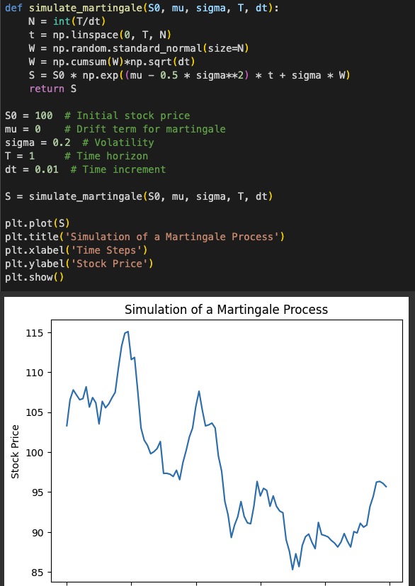
Sample Code for Simulating a Martingale Process

import numpy as np
import matplotlib.pyplot as plt

def simulate_martingale(S0, mu, sigma, T, dt):
    N = int(T/dt)
    t = np.linspace(0, T, N)
    W = np.random.standard_normal(size=N)
    W = np.cumsum(W)*np.sqrt(dt)
    S = S0 * np.exp((mu - 0.5 * sigma**2) * t + sigma * W)
    return S

S0 = 100  # Initial stock price
mu = 0    # Drift term for martingale
sigma = 0.2  # Volatility
T = 1     # Time horizon
dt = 0.01  # Time increment

S = simulate_martingale(S0, mu, sigma, T, dt)

plt.plot(S)
plt.title('Simulation of a Martingale Process')
plt.xlabel('Time Steps')
plt.ylabel('Stock Price')
plt.show()

This code simulates a martingale process for a stock price, assuming zero drift (( \mu = 0 )), characteristic of a martingale in risk-neutral measure.

Key Takeaways

Understanding the interplay between martingales, mean reversion and delta hedging is essential in financial modeling. It's important to recognize that certain stochastic structures are incompatible due to their underlying mathematical properties. Utilizing AI tools and programming can enhance the practical application of these concepts, offering dynamic ways to simulate and visualize complex financial processes.

References

• Hull, J. C. (2014). Options, Futures, and Other Derivatives (9th ed.). Pearson Education.
• Shreve, S. E. (2004). Stochastic Calculus for Finance II: Continuous-Time Models. Springer.
• Lewis, A. L. (2001). A Simple Option Formula for General Jump-Diffusion and Other Exponential Lévy Processes. Finance and Stochastics, 7(1), 1-14.